
 Figure1The "Beaming Frequency" is where curved line‑source behavior strays from straight line‑source behavior. Line arrays are hybrid solutions that exhibit both straight as well as curved line‑source behavior.
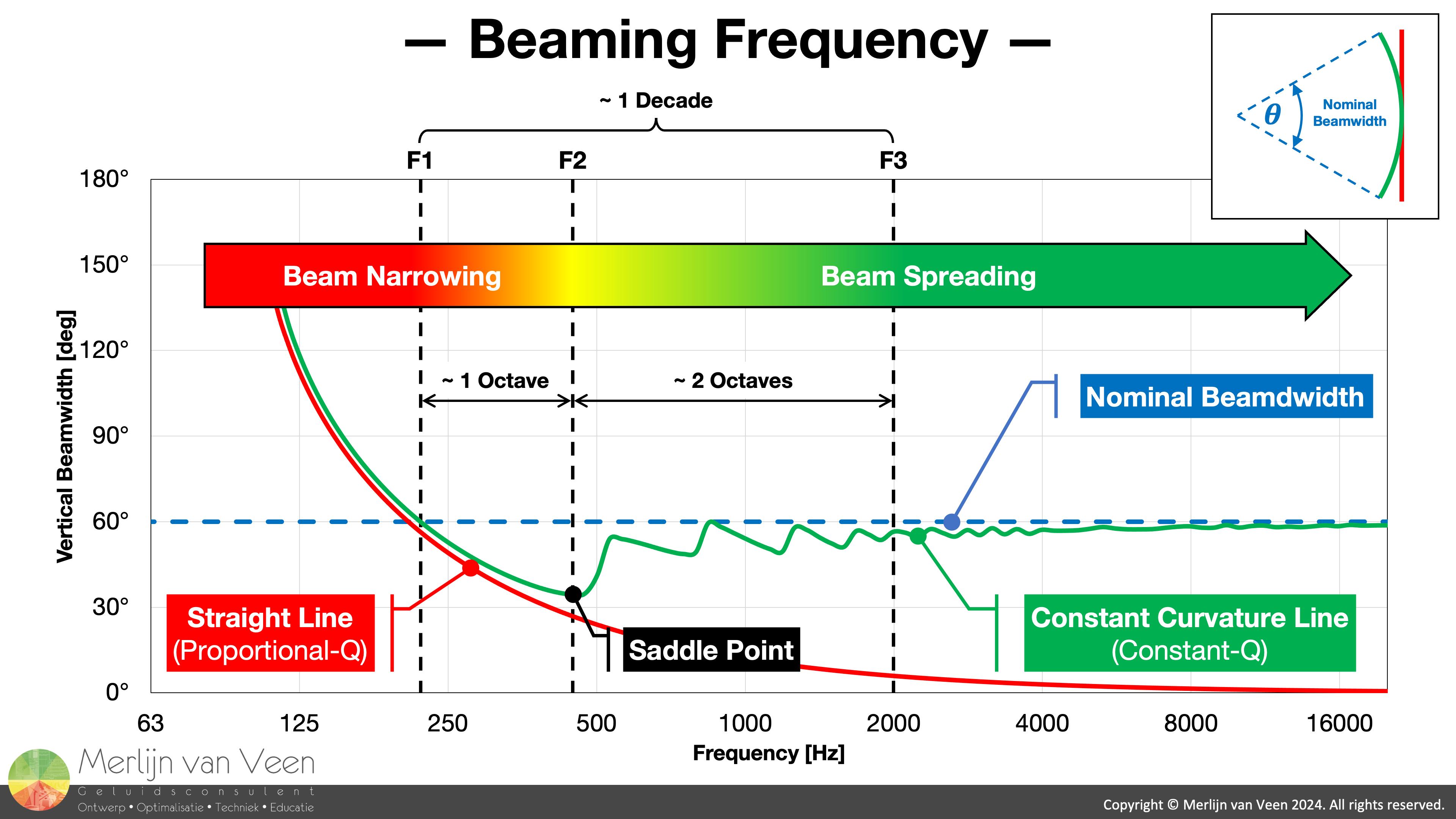
The former causes Proportional‑Q — in the vertical plane — whereas the latter Constant‑Q. And there will be an inevitable frequency span where one behavior transitions into the other. During which vertical beamwidth will narrow, by as much as one‑third less than nominal. The frequency where vertical beamwidth is at its narrowest is historically known as the "Beaming Frequency".
Figure 1 shows the — vertical — beamwidth, as function of frequency, for straight and constant‑curvature continuous line‑sources of the — same — length. The straight line‑source's beamdwidth (shown in red) narrows with increasing frequency. With each octave‑increment it is halved. Directivity factor \(Q\) is inversely proportional to coverage angle, i.e., beamwidth. And since beamwidth decreases with increasing frequency, \(Q\) — rises — with increasing frequency. Hence Proportional‑Q (\(Q\) is proportional to frequency).
The constant‑curvature line‑source (shown in green) — at first — follows the same progression. But come saddle point, its beamwidth starts to diverge. While the straight line‑source continuous to narrow (Proportional‑Q). The constant‑curved line‑source begins to spread and converges towards nominal where it becomes Constant‑Q. At the saddle point, the vertical beam — for curved arrays — is the narrowest. Hence "Beaming Frequency".
Figure 1 shows that for lower frequencies, up until the Beaming Frequency, line-sources — curved and straight alike — in general exhibit Proportional‑Q behavior. Whereas for higher frequencies — curved arrays — do respond to inter‑element splay. And effectively become "point‑and‑shoot".
Analysis
While being familiar with the phenomenon from other publications (H. Olson, etc.), the author first read about the — term — "Beaming Frequency" in product collateral1 from the early 90s. But failed to reconcile the published equations with the published values. As such, the author ended up doing his own preliminary — far‑field — analysis. And adopted the same major milestones' labels.
The lowest frequency \(F1\) where vertical beamwidth equals nominal:
\begin{equation}F1\approx \frac{21\times 10^3}{l\times \theta^{0,935}}\end{equation}
The beaming frequency \(F2\) where vertical beamwidth is roughly one‑third narrower than nominal:
\begin{equation}F2\approx \frac{42\times 10^3}{l\times \theta^{0,935}}\end{equation}
The frequency where vertical beamwidth recovers back to nominal \(F3\):
\begin{equation}F3\approx \frac{189\times 10^3}{l\times \theta^{0,935}}\end{equation}
For all three equations \(l\) is line length in meters. And \(\theta\) is the nominal — constant‑curvature — coverage angle (read: total splay) in degrees.
\(F1\) and \(F2\) are spaced roughly one octave appart (Figure 1). Whereas \(F2\) and \(F3\) about two octaves. Subsequently, the entire transition lasts about one decade.
In all instances, the major milestones' frequencies are — inversely — proportional to line‑length and nominal coverage angle. So either making the array longer or wider will lower the beaming frequency as well as all other milestones. Figure 2
Figure 2 shows an overview for different coverage angles (columns) and various line lengths (rows). Notice (as forecast by the equations) that the Beaming Frequency drops for both longer or wider arrays.
Direction of The Beaming Frequency
The direction of the Beaming Frequency — with respect to overall array‑orientation — is easy to forecast. The Beaming Frequency lives along the trajectory where there is — the least phase offset — between array elements. And source‑receiver path‑differences are minimal. 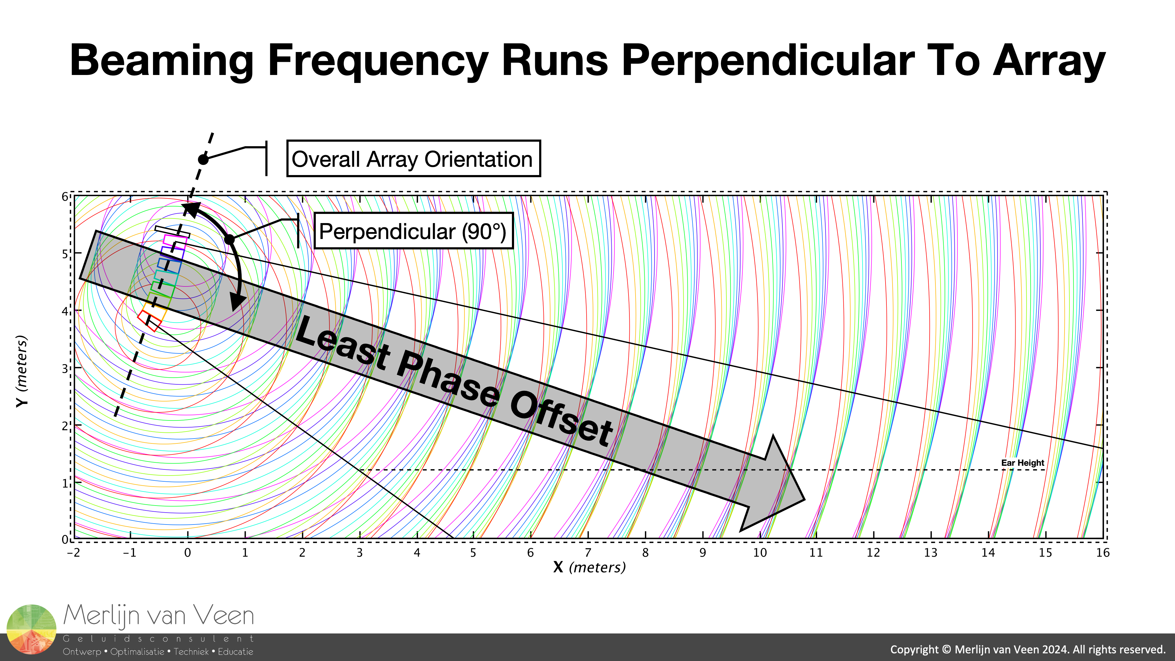 Figure 3If we do a quick ripple‑tank exercise (Figure 3), one clearly sees that roughly along the perpendicular (to the array) all ripples' crests intersect, i.e., are most in phase. Whereas everywhere else there is "coordinated" chaos.
Whether or not array‑elements will actually interfere; depends on whether their — vertical — coverages overlap. For which one can fall back on a tried and tested rule‑of‑thumb that states that a piston driver's (axial) coverage angle — exceeds — 90° for all frequencies whose wavelengths are longer than the driver's diameter.
For example, below 2 kHz for a 6.5" driver. Down to below 800 Hz for an 18" driver. In fact, individual piston drivers also exhibit Proportional‑Q behavior which is worthy of a separate article.
Suffices to say, the individual elements of small and large arrays alike — for the frequency‑ranges of interest — are effectively overlapped.
Where the Beaming Frequency ultimately falls, i.e., within operating range or not. And where the Beaming Frequency touches down within the audience. May audibly affect tonality throughout the audience.
In order for tonality to be preserved with increasing distance — all — frequencies need to loose market share at the same rate. However, when vertical beamwidth is a function of frequency, preservation of tonality over distance is compromised.
Tonal Implications
There are many use‑cases beyond the scope of this article that are worthy of separate consideration. For now, the author will limit to two typical scenarios. A short and a long array covering a level audience.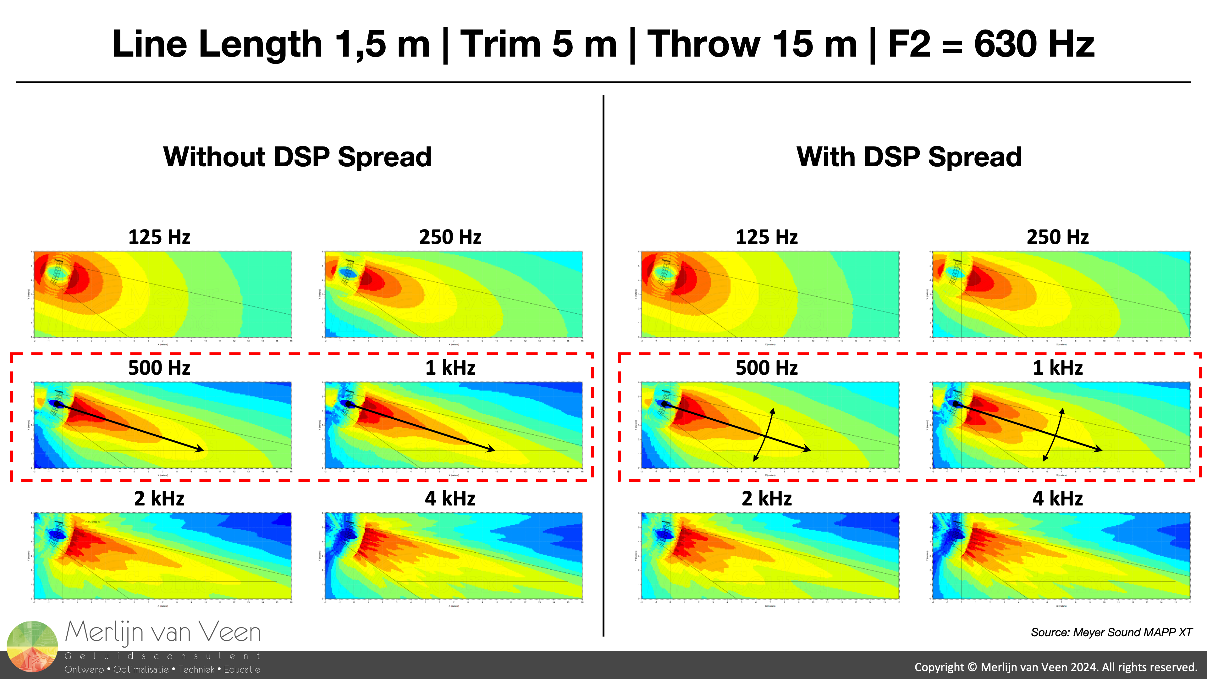 Figure 4Figure 4 shows a short array. For its given length and total splay, the "beamy" frequencies occur throughout the decade centered at 630 Hz. Right in the middle of its operating range while leaving lows and highs unaffected.
Notice in the left‑hand side of Figure 4 (without DSP spread), that both 500‑hertz and 1‑kilohertz beams are — too narrow — and overshoot the audience start. Followed by doing a nose‑dive halfway into the audience. Whereas all remaining frequencies are louder in the front and taper off towards the back.
Here the challenge becomes to redistribute the energy from a region where there is too much — the middle — to a region where there is too little; the audience beginning. Which can be achieved by, e.g., spreading the beam electronically — solely for beamy frequencies — by virtue of signal processing (right‑hand side of Figure 4). Figure 5Whereas Figure 5 shows a long array. For its given length and total splay, the "beamy" frequencies occur throughout the decade centered at 125 Hz. Concerning solely lower operating‑range frequencies while leaving mids and highs unaffected.
Notice in the left‑hand side of Figure 5 (without DSP lift), that both 125‑hertz and 250‑hertz beams, while being sufficiently narrow, due to their perpendicular orientation — land in the wrong place — i.e., first audience half as opposed to the last row.
Here the challenge becomes to redistribute the energy from a region where there is too much — first audience half — to a region where there is too little; the last row. Which can be achieved by, e.g., lifting the beam electronically — solely for beamy frequencies — by virtue of signal processing (right‑hand side of Figure 5).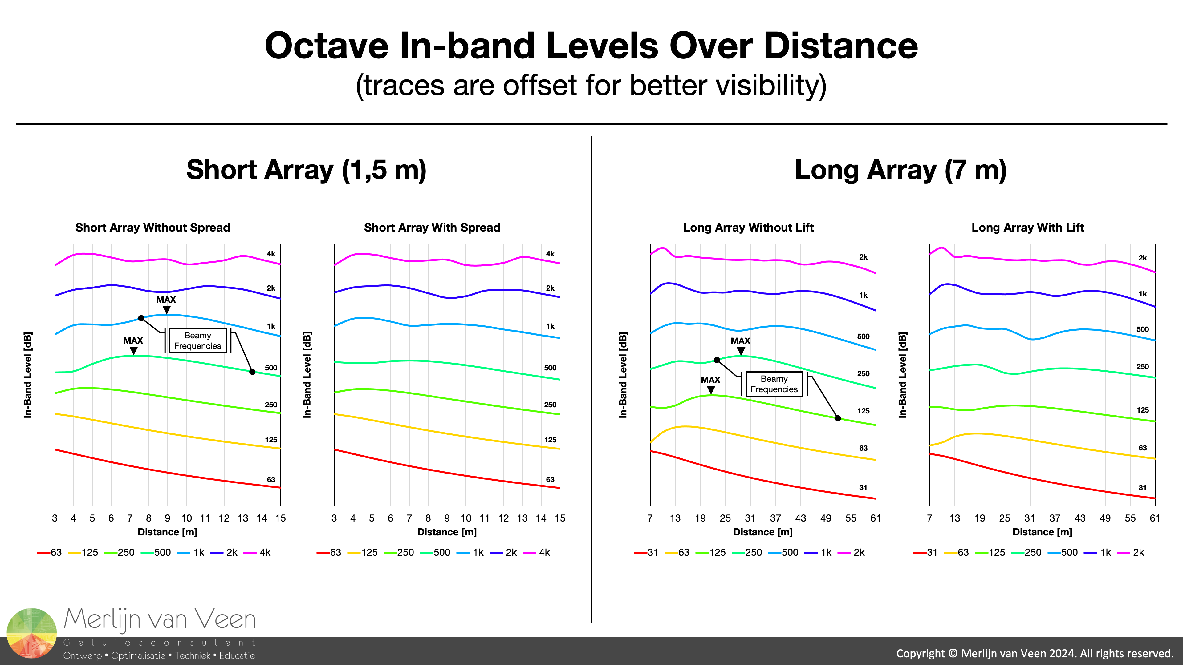 Figure 6Figure 6 shows octave in‑band levels over distance. Where the traces have been offset for better visibility. Notice in both cases that — without signal processing — not all frequencies drop in level with increasing distance.
Without signal processing, the beamy frequencies gain in level first while all remaining frequencies either maintain their level or taper off. A guaranteed recipe for tonal variation. Whereas with signal processing, by and large, all frequencies are louder at first and taper off towards the back.
Conclusion
All arrays — without additional signal processing — will manifest this phenomenon. And handling the beamy frequencies is essential for minimizing tonal variation throughout the audience. They cannot be remedied with equalization, since the root cause is a frequency‑dependent time‑problem. Which requires a "time" band‑aid as opposed to a "level" band‑aid like EQ or gain.
Further Reading
To understand why equalization is the wrong treatment — and will make things worse — please consider reading my article Pick your battles.
To understand why both array's lower frequencies exhibit point‑source behavior (6 dB per distance‑doubling) while mid- and high‑frequencies exhibit behavior — reminiscent — of cylindrical waves (3 dB per distance‑doubling), please consider reading my article Cylindrical Waves: Hyped or Not?
References
1. L‑ACOUSTICS V‑DOSC Operator Manual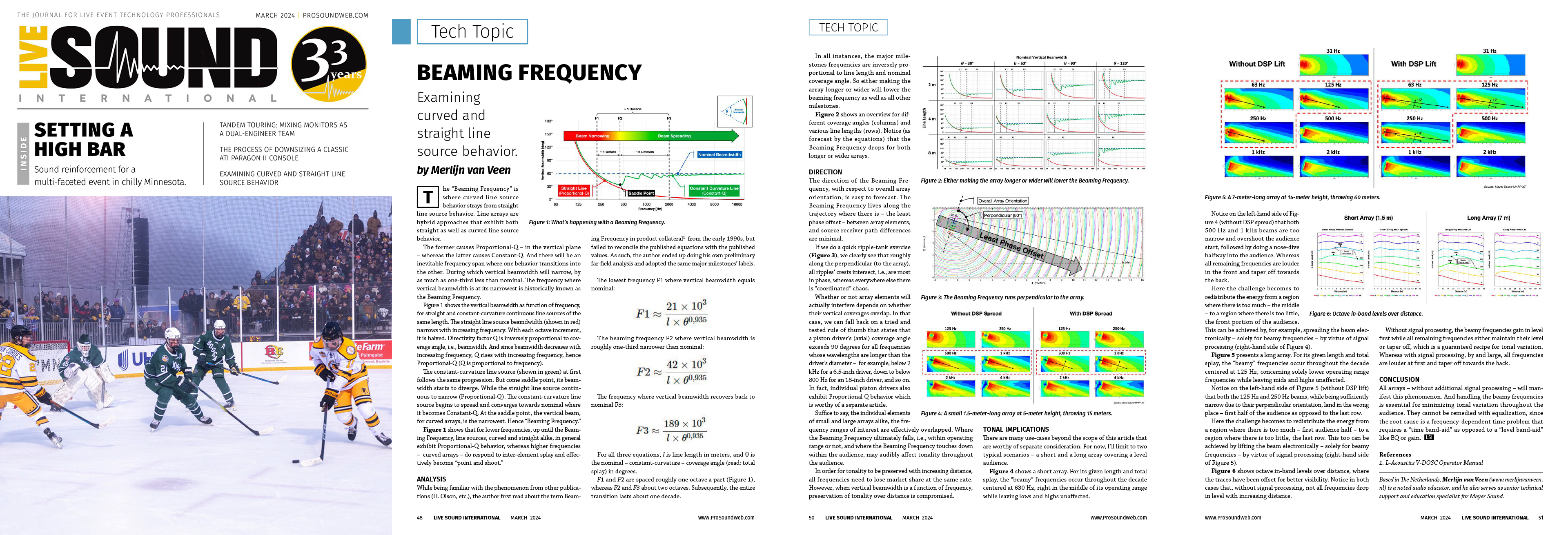
This article is also featured in the March 2024 issue of Live Sound International magazine.